setiQuest tutorial

The setiQuest project was spawned by Jill Tarter's TED wish and is sponsored by the SETI Institute. The goal is to empower "Earthlings" all over the planet to help in the Search for Extraterrestrial Intelligence. Their plan to do this is by allowing access to data collected from the Allen Telescope Array (ATA) and by releasing their source code sometime in Q3 2010. Access to the data was made available in April 2010. Source code is great but the true value of setiQuest comes from access to the data.

Today you can use the baudline signal analyzer to explore the setiQuest data. To get access to the data you'll first need to register for a free setiQuest user account. Next you will need to feed the data into baudline and that is the purpose of this tutorial.

There are two ways to get the setiQuest quadrature .dat files into baudline. One is to read them in as a raw data file. The other is to stream them into baudline's standard input (stdin) which is like recording from a microphone but instead using a Unix pipe construct.


raw data file
First thing you'll want to do is set the FFT size to 65536 since these are weak signals. Second, set the Open File window to use the Raw format and then select and open your data file. Next, set the Raw Parameters to the appropriate 8-bit quadrature format. Here is a screenshot of the proper setiQuest raw parameters:


Large data files are going to cause problems because baudline is basically a big RAM based buffer. You will need a lot of RAM and even then they will be clamped at a 2 GB limit. So opening in raw mode is good for small files but very bad for huge files.


stdin
This is the preferred method. Stream the .dat file(s) into baudline using the Unix standard input. This way you can record and pause just as if you had access to the live ATA data stream (as if it was a soundcard). With files and stdin you can process data at the speed you want and at the speed your computer can handle. Fast enough computers can actually record and have scrolling baudline spectrograms in real-time (8.7 MS/s quadrature). Here is a sample command line I use to stream setiQuest data into baudline:

cat 2010-01-22-kepler-exo4-1420mhz.dat | baudline -session setiquest -stdin -format s8 -channels 2 -quadrature -flipcomplex -samplerate 8738133 -fftsize 65536 -pause -utc 0

Here is a typical screenshot:


The large green window is the spectrogram display with frequency across the horizontal axis and time on the vertical axis. Vertical lines are constant tones. Sometimes you will see signals moving around in the spectrogram display; pulsing, drifting, wandering, ... The spectrogram display can be scrolled, zoomed, and controlled in numerous other ways.


Record, Pause, and Play
Use the 3rd mouse button (right button or Command+button) to popup the main menu and select between Record and Pause modes. You can also do this with the controls from the Play Deck. The idea is to record and watch the spectrogram scroll by and then pause it if you see something interesting or if you would like to perform some zooming, scrolling, measuring, or additional analysis.

Baudline has many features that can be used to analyze the data. Remember that the full power of baudline is accessed through the main popup menu. Some of baudline's many other windows have popup menus too.


Decimate and Down Mix
The Input Devices window is used for selecting the sound card and it also works with standard input. The Decimate By and the Down Mixer controls will allow you to zoom into the frequency spectrum much like how a radio tuner works. Decimation adjusts the sample rate so think of it as a way to change how wide a chunk of frequency you want to look at. Decimation is a great way to increase SNR similar to increasing the FFT size. The Down Mixer selects the frequency to look at just like a tuner dial on a radio.

These controls only work while in the record mode on the incoming data stream. So you can make changes while recording but if you want to change the entire data stream from the beginning you will have make the adjustment, exit baudline which will save your session settings, and then restart baudline from the command line.

I like running several instances of baudline with the same stdin data stream all at the same time. Setting decimation to none will give you the full width of the spectrum. I like doing this as a first pass and keep it around as a map for a second instance of baudline on another screen. I decimate and down mix in that second instance of baudline. Sometimes I have up to ten baudlines open at a time doing different things, managing memory usage is important when I do this.


Scroll Control
As its name implies, the Scroll Control window is how you control scrolling and manage memory. Baudline is basically a big wrap-around buffer and with this Scroll Control window you control the overlap value, the maximum capture time, and the amount of RAM to dedicate to buffer space.

The overlap setting adjusts the recording mode's scrolling speed. Fast on the left and slow on the right. Don't use it to change the size of the spectrogram image, instead use the timebase zoom controls for that. For setiQuest data I recommend setting the overlap to its maximum 1.0 value. This will let you collect the longest duration of data in the buffer. It will also slow the scrolling rate down so that your computer can better keep up with a real-time stream.

The buffers (MB) slider allows you set the maximum amount of RAM in megabytes that you want baudline to use. Big buffers allow for collecting large amounts of data and for fast timebase spectrogram zooming but they take up a lot of space. Too much RAM allocated means less is available to other applications and the operating system. When RAM gets low things can get slow when memory starts getting swapped to disk. My advice is to use a large buffer when you need to collect a lot of data or for a long time. Use smaller buffers for things like when you decimate by 4096.

The Reallocate Now button will erase all the current data in and reallocate the buffers according to your new overlap and MB settings. Pressing this button will also update the Maximum Capture Time value. Use this button with caution.


Color Aperture
Weak signals have very little dynamic range so the Color Aperture window is a way to control spectrogram intensity.
Adjust the upper and lower dB values to match you signal's spectral range and maximize your color resolution. Heavily averaged (integrated) signals have a lower variance so the upper and lower controls can be set much closer together without the color clipping.


Average Spectrum
The Average window allows you to integrate (average) a large number of spectral slices. Spectral integration reduces the variance of the noise floor which is useful for seeing weak signals. Zooming into the Hz and dB axis is also very useful for seeing weak signal details.


The Average window operates in the record mode by the on/off collecting of data and in the pause mode by copy-n-pasting chunks of data. The Average window has a number of other useful features such as multiple color spectral traces (F# banks) and exponential decay while recording. These controls are accessed by the Average window's popup menu (3rd mouse button).


Histogram
The Histogram display shows the probability distribution of a waveform's sample amplitudes. The setiQuest data is predominantly noise that has a Gaussian shaped distribution (bell shaped curve). The unusual example histogram below shows the basic Gaussian shape with an offset between the I (green) and Q (purple) quadrature channels.

Normally the I/Q channels are perfectly balanced and all that is visible is a clean Gaussian shape that is the color cyan which is the sum of green and purple. Here is another Histogram window example that shows distribution gaps due to the signed 8-bit quantized samples. Note that 2^8 = 256 samples.

The Histogram window is useful for seeing certain types of signal distortions and collection artifacts but it is not useful as a weak signal analysis tool.


Drift Integrator
The Drift Integrator window is a powerful but more complicated set of controls for all things integration related. The beam width control is like averaging for the spectrogram display. The drift rate and Auto Drift controls are tightly coupled to both the Average window and the Spectrogram display.

I recommend setting the "anti-alias on spectrogram zoom" setting as it will dynamically improve your spectrogram image when you zoom out. The rest of the Drift Integrator settings have a great deal of potential for SETI but they are slightly dangerous so they are for experts only. Read the online manual and become an expert!


More
I've tried to make the setiQuest AMC-07 and the Kepler Exoplanet 4 blog posts as educational / tutorial-like as I can while still reporting useful analysis. I describe all the details and settings that I used so anyone should be able to reproduce my results. Many baudline tips and DSP techniques are hidden within too. I hope you find them helpful.

setiQuest Kepler-Exo4 1420 MHz

This analysis is of the setiQuest Kepler Exoplanet 4 data file with the baudline signal analyzer. The quadrature data file has a base frequency of 1419.4464 MHz and a sample rate of 8.738133 Msamples per second. Not much information is given about this data file but I assume it is an observation of the Kepler Mission satellite collected at the Allen Telescope Array. But the SNR is far too low to be the telemetry of a near Earth satellite so the signal source could be the Kepler-4 planet (KIC 11853905). Will need source confirmation from the SETI Institute since they collected the signal. In any case there is some interesting stuff happening in this data file.

The following command line was used to stream the Kepler Exoplanet 4 data file into baudline:

cat 2010-01-22-kepler-exo4-1420mhz.dat | baudline -session setiquest -stdin -format s8 -channels 2 -quadrature -flipcomplex -samplerate 8738133 -fftsize 65536 -pause -utc 0

Full 8.738 MHz view
The Kelper Exo4 file was streamed into baudline's standard input. A 65536 point FFT was used for a bin resolution of 266.667 Hz / bin. The Welch window was used for a little more signal extraction SNR. The Histogram window shows a nice Gaussian noise shape with even-odd holes for the 8-bit samples. Optimal anti-alias beam slices were used to smooth the spectrogram and the Color Aperture window was tweaked to maximize the color resolution. Only 50 seconds of the spectrogram are shown because the run was RAM limited. The red Average spectrum shows a hump and 6 strong tones.


From the spectrogram; the two strongest features are the stationary tone at -3874 kHz and the spectral hump at 1000 kHz. Looking at the red Average plot shows several more sharp tones. Here is a list of the potentially interesting targets, add 1419.4464 MHz base frequency:

• -3868800 Hz - very strong - stationary
  
• -3470933 Hz - strong - random walk - drift
  
• -2713067 Hz - weak - wild random walk - drift
  
• -1482667 Hz - strong - wild random walk - drift
• +586133 Hz - strong - drift - extremely interesting - "friend"
  
• +977867 Hz in hump - weak - wild random walk - drift
• +900000 ... +1111000 Hz (hump) - hydrogen - see below
  

All of these candidate signals are investigated individually below. Decimating by 4096 to increase the extraction power was used for all of them expect the hydrogen hump. Most of the analysis is quickly skimmed over except for the most interesting +586133 Hz signal which is analyzed at the end.


Hydrogen and Friend
Zooming the Average window into the frequency axis reveals this strong tone and spectral hump. Tone and hump, they make an interesting pair.


The spectral hump at +1 MHz is hydrogen. Interstellar hydrogen in space emits radio frequencies at 1.42 GHz, so with the base frequency offset the hump is centered at around 1.421 GHz. The strong tone to the left is just outside the "water hole" and because it requires a much more detailed analysis we will investigate it last.


-3868800 Hz
Decimating by 4096. Very strong stationary tone in the filter roll-off skirt. No drift. Not interesting.



-3470933 Hz
Decimating by 4096. Random walk tone with positive slope drift. +29 Hz drift / 326 seconds = +0.089 Hz / sec.



-2713067 Hz
Decimating by 4096. Random walk tone with positive slope drift. Difficult to measure, roughly +29 Hz drift / 326 seconds = +0.089 Hz / sec. It looks a bit like the previous signal but it is much weaker and it appears to be jumping around more. It could be a sideband of something but it doesn't seem to be harmonically related to the previous tone. More decimation might help pull out more signal.



-1482667 Hz
Decimating by 4096. Random walk tone with positive slope drift. Difficult to measure, roughly +29 Hz drift / 326 seconds = +0.089 Hz / sec. Looks almost exactly like a stronger version of the above signal.



+977867 Hz
Decimating by 4096. This signal is the weak tone that is in the hydrogen hump mentioned above. Very weak version of the above signal. Strength and random wander are almost identical to the -2713067 Hz signal. Why this signal is in the hydrogen hump is unknown.

This and the previous two signals are virtual copies of each other. They do not appear to be harmonically related. They could be sidebands or distortion products of the strong stationary tone but the harmonic relationship doesn't seem correct.


+586133 Hz
"Hydrogen's friend." This signal is extremely interesting. The true frequency of this tone is 1420.586133 MHz and it is just to the left of the hydrogen spectral hump. To zoom into the +586223 Hz tone the Input Devices window was set to decimate by 4096 with a +30 dB gain to improve the quantization SNR.¹ The down mixer was set to a center frequency of +586133.3 Hz. The 4096 decimation along with a 65536 point FFT resulted in a bin resolution of 0.0651 Hz / bin.


The red spectrum in the Average window shows a strong +15 dB tone at +586223 Hz. The Histogram window shows the noise to have a nice Gaussian shaped curve. The Gaussian window was used to improve the spectral time resolution. The Color Aperture window was set to a -27 ... -61 dB range to improve the color resolution of the spectrogram. The green spectrogram window shows what previously was a constant stationary tone is now a drifting signal that has a slight random walk. Note that the spectrogram's horizontal zoom has been changed to Hz=1X. Here is a full screenshot:


Making some measurements in the spectrogram window shows that the +586223 Hz signal has a drift of +4.30 Hz / 326 seconds = +0.0132 Hz / second. It starts as what looks like a random walk as the tone zigzags back and forth. Then something really interesting happens half way down, it looks like the signal is being modulated. Zooming in on the lower half and increasing the Gaussian beta value to 11 shows: (click on image for higher resolution version)


This looks like FSK modulation with the delta between mark and space frequencies being about 1.2 Hz. Below is the Average spectrum showing the mark and space frequencies:


The purple spectrum is from the beginning of the modulated section. Since the signal is drifting with a positive slope the mark and space frequencies move to the right. The green spectrum is from the mid/bottom of the modulated section. This is clearly 2-tone FSK but at an extremely low baud rate with a very close mark and space frequency delta.


Enhance Resolution
The new blip Fourier transform enhances spectral resolution which is ideal for deep zooming down to the sample level. Time, frequency, and phase details are improved by using a new analysis primitive called the blip(let). A focus parameter allows for algorithm fine tuning on a signal by space by zoom basis.

Zooming into the FSK signal using a second decimation pass for a total decimate by ratio of 524288 and a bin resolution of 0.01628 Hz / bin. With focus=1 the structure of the individual FSK bits are clearly visible in the magnitude space view below:


Also part of the blip Fourier transform is a blind phase lock algorithm that tracks changes in phase. The problem of spinning phase that is inherent in the short-time Fourier transform (STFT) is solved with blind phase locking. Now the other half of the spectrum, the phase half, contains visibly useful information. With focus=4 the phase of the FSK bits are fairly constant in the unwrapped phase space view below:


The visible phase changes follow what is expected for a random walk coupled with FSK mark/space transitions. There is a fair amount of phase noise present but it does not appear that any phase coding exists within the steady state or the bit transitions.

In the spectrum section above the dB axis is incorrect. Since this is phase space the units should be {-pi ... +pi}. This will be fixed in a future version of baudline.

Also note that the spectrogram timebase parameter for the above images was set to 3X. The overlap value was 1 so this means that baudline can zoom in three more scale factors before the digital bottom is reached at the discrete sample level.


Demodulation
Since the entire FSK signal is drifting somewhat randomly at about +0.0132 Hz/sec machine demodulation is a bit difficult. Backed decimation up a notch from the previous Enhanced Resolution section since the following demodulation works better with a little less zoom. Used a second decimation pass, like was done previously, for a total decimate by ratio of 262144 and a bin resolution of 0.03255 Hz / bin. Baudline's periodicity bars were used to place and fine tune a horizontal grid that perfectly matched the modulated FSK symbols. See the two slightly overlapped spectrograms that have the periodicity bar overlays below: (click on image for higher resolution version)


Note that FSK2 modulation has one symbol per baud. From the periodicity bars delta selected value the baud rate was measured to have a period of 1.976 seconds which is 0.5061 baud. This works out to a spectral efficiency of roughly 0.17 (bit/s)/Hz.² The periodicity bars sliced the symbols perfectly. With the periodicity bars up I was able to manually demodulate the individual bits. Here are the demodulated bits, it begins with a large number of leading zeroes:

00000000000000000000000000000000000000000000000
10100010001010101010010000000000101010101001010
10101010101010101010101010010101010101010101010

In an attempt to make some sense of this bit stream here are the demodulated bits in a reduction grammar notation:³

0* 2(10) 00 1(10) 00 5(10) 0 1(10) 9(0) 5(10) 0 15(10) 0 10(10)+

where the 0's and 1's are bits and the bit string in parenthesis is repeated by the number before it. The pattern is mostly repeating 10's interspersed with an occasional 0 or two.

Ignoring the leading zeroes, here is the bitstream broken down into 32-bit hexadecimal integers (big endian):

10100010 00101010 10100100 00000000 = 0xA22AA400
10101010 10010101 01010101 01010101 = 0xAA955555
01010101 00101010 10101010 101010.. = 0x552AAAA.

There are 55 zero bits and 39 one bits which is somewhat lopsided but the sample size is way to small for that to be significant. It is interesting that there is not a single run of ones (11) in the bit stream which would suggest some form of Non-Return-to-Zero Inverted (NRZI) coding.⁴

The bit stream is definitely not random but I haven't been able to decode a pattern out of it yet. It is also possible that the demodulation process produced a couple of bit errors. It is also unfortunate that the data file terminated when it did. Plugging this bit stream (and parts of it) into Google returns zero hits. Maybe some bit wackers⁵ or crypto folk can pull meaning out of this bit stream.


Listen
The decimated quadrature FSK signal was mixed up to passband (real). To hear this signal download the kepler-exo4_FSK.wav file, load it into baudline, then open the Play Deck window to adjust the audio controls, and press play.


You can slow down the sample rate by adjusting the speed control or change the center down mix frequency by adjusting the shift control. Pressing the small arrow in the bottom right corner will pop down a section that has more controls. From there you can apply an equalization curve or adjust low and high pass filters to remove out-of-band noise.


Autocorrelation
The random walk wandering FSK signal was then ran through baudline's Autocorrelation transform. The Autocorrelation transform shows the self similarity of a signal and it can also be utilized as a form of waveform trigger lock mechanism. Think of Autocorrelation as a sort of self syncing waveform raster display.

For reference the Color Aperture window parameters were set to upper=-48 dB and lower=-69 dB. All other parameters except the windowing function are default. The Kaiser window was used and the beta parameter was increased from 0. to 15. in steps to create the following Autocorrelation spectrogram images:

beta = 0. (square window)

beta = 5.
beta = 15.

The progression of the Kaiser beta value shows how the structure evolves as the window gets narrower. No beta value here is inherently correct but the structures seem to stabilize with the higher betas.

Here is an Autocorrelation movie of the variation of the Kaiser window beta. Notice how patterns and structures pop out of the noise as the beta parameter changes. The audio in the movie is the sound of the drifting random walking FSK signal that has been speed and frequency shift modified for the audio band. Make sure to watch this in fullscreen 720p HD so you can see all the details.



This is not random noise and this is not what the Autocorrelation of a random walk looks like. I was expecting to see the FSK bits flipping on and off from a synchronized waveform perspective. That didn't happen and what this is is a lot more than 94 bits worth of structure. Also the drifting random walk isn't random at all, it contains information. What I believe is happening is that the drifting random walk and the FSK bit stream are modulated together to create this image. I've never heard of a modulation scheme like this before. It does have elements of NTSC and Hellschreiber to it but at an extremely low data rate.

I tried different FFT sizes and different time domain operations from the Input Mapping window that cause various signal distortions. The basic image structure did not change. This tells me that the signal is fairly robust and not an artifact created by the analysis equipment.


Conclusion
The importance of this analysis depends greatly on the identity of the target source. Is it the Kepler satellite, the Kepler-4 planet, or something else? It is very unlikely an error in the collection or analysis caused the modulated bit section because other features in this data file are stationary or drifting differently. It is extremely unlikely that the modulated bits were created by natural phenomena. Decoding of the bit stream may prove enlightening in identifying the source. The Autocorrelation images are likely an interesting byproduct of the FSK data stream coupled with the drifting random walk.

I really don't know what to say or think at this point. The SETI Institute collected this signal and they, hopefully, will tell us what the celestial source is. [Update: This thread confirmed the signal source to be the Kepler 4b star.]

Some important questions about the FSK modulated signal:

• Is the signal's proximity of -500 kHz to hydrogen significant or is it an aliasing artifact?
• Are the other tones related in any way? (harmonically or temporally)
  
• Why is the signal drifting at a +0.0132 Hz/second rate? What should it be drifting at?
• Why is it undergoing a random walk?
• Why are the mark and space frequencies so close together? (1.2 Hz)
• Why is the 0.5061 baud rate so low?
• Do these modulation parameters match any known modem or system?
  
• Do the demodulated bits match any known line coding, preamble, or training sequence?
• Why is there not a single run of ones (11) in the bit stream?
  
• Are there any "interesting" sequences or patterns in the demodulated bits?
• Is there any significance to the Autocorrelation images?
  
• Will this signal ever be seen or collected again?
  

Does anyone have any answers or ideas?

[Update: The SETI Institute did a re-observation of the Kepler-4 target and the analysis report is here setiQuest Kepler-4b redux.]

Footnotes
1. Decimating by 4096 has the effect of increasing SNR but with the byproduct of reducing gain. Since baudline uses a 16-bit internal sample size this gain reduction can push any weak signal past the LSB thus truncating it. The +30 dB decimation gain setting improves the quantization SNR which eliminates the potential signal loss problem. Note that SNR has been used twice here in this note but in different contexts.
2. This spectral efficiency is roughly equal to that of a 110 baud Bell 101 FSK modem.
3. A context-free grammar is a Computer Science tool that is used to define a formal language. They are very useful in the design of finite automata. Their reduction ability can simplify a complex repetitive string down to it's basic structure.
4. Non-return-to-zero (NRZ) is a telecommunication line coding technique that is useful for overcoming channel deficiencies and for dealing with clocking or synchronization issues.
5. Yes, "bit wacker" is a technical term.

setiQuest amc7-3693.4464 MHz

Using the baudline signal analyzer to browse the setiQuest 2010-04-02-amc7-3693.4464 data file. It took most of a day to download the 3 parts of the amc7 data files (5.7 GB) and combine them. This radio telescope data file is way too big to load so it had to be streamed into baudline. Two benefits of streaming to standard input are that you can see the recorded signal data scroll by and that the Input Device's "decimate by" feature can be used to further increase the signal extraction power.

The following command line was used to stream the 5m 26s quadrature setiQuest signal into baudline:

cat ~/setiquest/2010-04-02-amc7-3693.4464-8bit_combined.dat | baudline -session setiquest -stdin -format s8 -channels 2 -quadrature -flipcomplex -samplerate 8738133 -fftsize 65536 -utc 0 -pause

Full 8.738 MHz view
Switching baudline to the record mode allowed the standard input to be collected and displayed. The red Average window reduces the variance of the noise floor and lets weak signals stand out. The green spectrogram is a time vs. frequency plot which shows the presence of several constant tones (straight lines). The Histogram window shows a Gaussian curve (see AWGN) which is customary for noise sampled from an analog digital converter (ADC), notice the alternating blank vertical lines caused by the signed 8-bit sample format. The Color Aperture window allows the upper and lower spectrogram intensity limits to be adjusted for maximum visual sensitivity. See the screenshot below (click for a larger image):


A 65536 point complex FFT was used for display and analysis. The frequency axis was zoomed in to a Hz=1X resolution to focus on the tones at +500 kHz. The screenshot of the zoomed in Average window is below:


The main tone is at 473 kHz with several weaker distortion sidebands. Next we want to zoom in even more to see what is going on.


Decimate by 512
The decimation and down mixer feature in the Input Devices window was used to zoom into the frequency axis which also has the side benefit of increasing the signal's SNR. Decimation by 512 was done combined with a 65536 point FFT which has the equivalent extraction power of a 32 million point FFT. This works out to a bin resolution of 0.52 Hz / bin. The down mixer is a digital down converter (DDC) which works a lot like turning a radio tuner. The down mixer was set to be centered on the strong tone at +473 kHz by setting the frequency range to +464533.3 ... +481600.0 Hz.

Interesting side note is the 8.3 Msample calibration rate estimate for stdin. The sample rate estimate is a clock measurement of the speed baudline is collecting data, in this case from stdin. This means that baudline is collecting standard input data from a file, decimating, down mixing, calculating a 65536 point FFT, accumulating the Average window, calculating and drawing the sample Histogram, and rendering the scrolling spectrogram in almost real-time on a cheap $500 one-year-old 2.0 GHz Intel Core 2 Duo machine.

Next, the "transform cache" feature was enabled in the Drift Integrator which used 524 MB of RAM to cache the results of the 65536 point FFT for extremely fast frequency axis zooming and scrolling. The Drift Integrator has a number of other useful features such as beam slices, Auto Drift, a folding paste algorithm, and anti-alias on spectrogram zoom which I will explain in a future blog post.


Below is a full screenshot of the result of the decimation and down mixing:


The red Average spectral plot and the green spectrogram show the same range of frequency data but at different Hz scale factors. The strong tone at 473067 Hz and its sidebands are the main concern of interest here. Notice the first sidebands offset by ±979 Hz on both sides of this strong 473 kHz tone are wiggly. Next we will zoom in on one of them.


Zoom Hz=1X
The Command+Left key was pressed several times to change the spectrogram's frequency zoom factor from 32X to 1X. Since the "transform cache" was enabled the zooming and frequency scrolling was extremely fast and responsive. It was like exploring the spectrum with a real-time DSP microscope looking for interesting spectral features. A screenshot of the wandering tone (F2) at 472075 Hz is below:


It was interesting to discover that the sidebands, offset by ±979 Hz, are mirror images of each other. The sidebands (F2) are about 25 dB down from the main tone (F1). The third ±harmonics (F3) are also wandering mirror images of F2, the F4 harmonic is missing, while the F5 is a clean constant tone. Here is a screenshot of -F3:


The wandering -F3 tone is just a weaker version of -F2 with 2x the frequency stretch which is customary for harmonic progressions.

Amplitude modulation (AM) of the strong 473 kHz tone by an unknown signal would cause similar sidebands. They could be distortion products from the transmitter or the radio telescope collection equipment. The wandering looks like it could be oscillator drift of the ADC sampling clock but that is just a guess.

Let's move the frequency scrollbar to look at the strong 473069 Hz tone. Here is a screenshot of the carrier (F1):

It looks very stationary and popping up baudline's crosshair cursor verifies such at this magnification level.


Decimate by 4096
Let's zoom in a little more. Increasing the decimation factor to 4096 reduces the bin resolution to 0.0651 Hz / bin. Below is a spectrogram screenshot of the strong carrier (F1) at this increased frequency resolution:

The strong tone has a slight drift of +0.52 Hz over a course of 326 seconds. This is about equal to the bin resolution from the previous decimate by 512 case so it isn't surprising that the signal looked stationary in that view. The increased frequency zoom has made the signal start to look a bit wiggly. What we need is even more frequency resolution.


Decimate by 32768
Baudline has a maximum "decimate by" limit of 4096 so I used a 2-pass method of decimating by 4096, saving the file, then feeding that into standard input again but with a decimate by 8 factor. I call this multi-pass algorithm "decimate by ∞" where you keep taking the output of the decimator and feed it back into the input. You can keep doing this ad infinitum until you end up with zero samples. I could of kept decimating past 32768 but too much time information would of been lost from the spectrogram and resulted in a poor looking image. The bin resolution of decimate by 32768 is 0.00814 Hz / bin. The once stationary tone no longer looks straight in the spectrogram below:


The tone isn't just drifting, it also has an incredible amount of wander to it. I measure a top to bottom drift of +0.35 Hz over 326 seconds. This isn't surprising, zoom in deep enough and even the world's best oscillator is will have some variation but more likely you'll be seeing the error in the ADC clock!

I've seen this deep decimation frequency wandering before in this Mystery Signal.

For fun this is what the decimate by 32768 quadrature signal looks like in the Waveform view:

Note that most of the noise has been decimated away and a quadrature sine wave is visible. Nice 90º phase shift.


Conclusion
The combination of a large FFT and high decimation factor allow baudline to zoom in for a deep view of weak signal behavior. Using baudline's multiple features allowed for detailed signal measurements and interactive fast browsing of the time-frequency domain.

The setiQuest AMC-07 data file had several stationary tones with strong distortion sidebands. The wandering mirror sidebands are likely caused by oscillator drift of the ADC sampling clock. The non-drifting stationary nature of all tones in this data file suggest the source is of terrestrial origin.

[Update: This thread said that the signal is from the AMC-7 geosynchronous satellite.]

I joined setiQuest

I joined the setiQuest project that is being sponsored by the SETI Institute. As their blog states, today truly is an exciting day. The setiQuest project is placing data sets collected from the Allen Telescope Array into the public domain. Their goal is to encourage "citizen scientists" to help in the search for extraterrestrial intelligence by analyzing radio telescope data and look for signals. Here is a baudline screenshot of the one second test .dat file:


The red spectral plot of the Average window shows a strong tone at -469 kHz and two weaker tones at around -2 MHz. The slopes on the left and right of the red Average spectral curve are from filters in the sampling unit or from a digital down conversion (DDC) process. The slight negative slope (-0.5 dB over 6 MHz) of the spectral curve is interesting, I'd expect it to be symmetrical around 0 Hz but it could be because this chuck of spectrum was extracted from a wider section of bandwidth.

The green spectrogram plot shows that these tones are stationary for the one second file duration which is not long enough to determine if they are stationary or are drifting. I need to look at the larger 1.9 GB data file, that is still downloading, to know for sure. Looks like there might be some modulation but that could just be the noise. The tones are fairly weak signals and further analysis is required.

The histogram on the right shows that sample data has a Gaussian distribution which is to be expected from radio telescope data. The histogram is centered at zero and it doesn't have any skew which is good.

This one second test data file was streamed into baudline's standard input. The data format is 2-channel quadrature signed 8-bit samples. The sample rate was calculated by dividing the one second file size by 2 to be 8738133 samples/seconds. Here is the command line used:

cat 2010-04-02-amc7-3693.4464-8bit-one-second.dat | baudline -session setiquest -stdin -format s8 -channels 2 -quadrature -samplerate 8738133 -pause

So join setiQuest, download baudline, and start analyzing signals today.

Ferranti Mark 1 computer music

The BBC is reporting that it has unveiled the oldest known recording of computer generated music. This recording was generated by the Ferranti Mark 1 computer at the University of Manchester in the Autumn of 1951. The Ferranti Mark 1 was the first computer to have a memory device that allowed it to run software programs. Previous computers of the day ran hardwired programs which were much more difficult to program.

The baudline spectrogram visualizer created the image below of the historic Ferranti Mark 1 computer music:


There are two interesting spectral features visible in the spectrogram.

The first feature is the frequency folding at 1012 and at 2024 Hz. These mirror spectral images can be artifacts of a sample rate conversion with poor anti-alias filtering or they could be caused by modulation (AM or FM) of the audio output. Modulation is the likely explanation because the audio output is suspected to be a simple wire connection to one of the Ferranti's register bits. Toggling a register bit at a CPU clock frequency at about 1012 Hz could create similar modulation sidebands. The Ferranti Mark 1 had a standard instruction time of 1.2 ms and a multiplication instruction time of 2.16 ms which is near a 1 kHz clock rate. On a related note, mystery signal #4 has similar modulation side-banding and the Khoomei Acoustic Analysis blog post has similar frequency folding.

The second spectral feature of interest was discovered with baudline's harmonic measurement bars. The harmonics of the musical notes are all missing their fundamental frequency. The exact cause is not known but a phantom fundamental is not easy to generate by bit twiddling. An analog filter or the frequency response of the loudspeaker could have caused this fundamental removal. Diode rectification is not the cause because the |x| absolute value operation moves the fundamental and it also moves the harmonics. On a related note the musical output is monophonic and has an apparent one octave range.

For technical information about the Ferranti Mark 1 computer see:

• http://www.computer50.org/mark1/FM1.html

Cassini - Eerie Saturn Radio Emissions

The baudline scientific visualizer was used to investigate some eerie Saturn radio emissions captured by the Cassini spacecraft. NASA believes that the source of these radio waves are related to the auroras near the poles of Saturn. The 27 minute radio emission signal was collected by Cassini's radio and plasma wave instrument and has been compressed down to a 73.5 second audio file for playback.


This signal looks and sounds a lot like Earth VLF chorus with fading blobs of spectrum moving up and down in frequency. The large blocks visible throughout the spectrogram are interesting looking artifacts that could be synthesis or compression related. Another interesting artifact are the horizontal scan lines that can be seen in the zoomed in spectrogram image below:


The NTSC-like horizontal scan line artifacts could be synthesis based or they could be related to how the Cassini sensors operate. Baudline's periodicity bars measured the scan lines to have a repetitive spacing of 0.1487 seconds which when multiplied by the 5000 sample becomes 743.5 samples. Adjusting for a 73.5 second to 27 minute file expansion, a reciprocal factor of 22.04, the number of samples becomes 16386.7 samples which is very close to 16384 a power of 2 and a popular buffer size.

Fedora 8 vs. openSUSE 10.3 vs. Ubuntu 7.10

Linux live-CD's are a great nondestructive way of auditioning Linux. Simply pop a live-CD into your CD drive, reboot, and then in a couple minutes you are running Linux. No hard drive partitioning, no lengthy installation process, no fuss. Linux live-CD's are also a quick and easy way to try many different Linux distributions. The latest Fedora, openSUSE, and Ubuntu live-CDs were tested for compatibility with the baudline signal analyzer.

The following Gnome based Linux distributions were all released during October and November 2007 with live-CD versions:

• Fedora 8
• openSUSE 10.3
• Ubuntu 7.10

Since they were released around the same time, all three use very similar versions of the Linux kernel, X-Windows, Gnome 2.20, and other common libraries. So it seemed like a great opportunity to compare them and see how well they worked with baudline. In theory the 3 different distributions all should of behaved in about the same way but they didn't. Another fine point is that all three Linux live-CD's advertised Xgl compiz 3D window effects but unfortunately none of the distributions supported this on our two test systems with the default video card drivers. For a review of a 3D compiz desktop see this Kororaa Linux Xgl LiveCD review.

Test Systems
We used two different 4-year old machines for the tests just to make sure that some unusual behavior wasn't being caused by an odd poorly supported piece of hardware. Here are the machine specs:

• Intel Pentium IV 2.0 GHz
• VIA P4X266 chipset
• 512 MB RAM DDR266
• GeForce4 MX 440 AGP 4X video card
• Creative Labs Sound Blaster 16 PCI ES1371
• integrated VIA VT8235 audio chipset

and

• AMD Athlon XP 2600+ 2.1 GHz
• nVidia nForce2 chipset
• 1.5 GB RAM DDR333
• SiS 300 PCI video card
• Labtec-704 USB microphone

We performed a simple rendering benchmark that consisted of running baudline with the -reset flag, then recording a full buffers worth of data, pausing, adjusting the Color Aperture window as a remap tweak, and then measuring the FFT transforms/second value in the Stats window. This simple repeatable test caused baudline to re-render it's spectrogram which is a CPU intensive operation that involves the baudline, X-Server, and kernel code.

Now let the testing begin!

Fedora 8
RedHat's latest community release uses the Linux 2.6.23.1-42.fc8 kernel and the Xorg 1.3.0.0 server. Video defaulted to 24 bpp graphics and all the audio devices were found and enabled. Here is a screenshot of baudline running on Fedora 8:


The main font is wrong, it is bold and mono spaced, but it is readable. The incorrect font caused some of the baudline windows to have spacing and layout issues but this is purely cosmetic. The baudline spectrogram rendering test resulted in 4320 FFTs/second on the Intel P4 CPU and 8000 FFTs/second on the AMD Athlon CPU.


openSUSE 10.3
Novell's latest community release uses the Linux 2.6.22.5-31-default kernel and the Xorg 7.2 server. Video defaulted to 16 bpp graphics and none of the audio devices were found or enabled. Here is a screenshot of baudline running on openSUSE 10.3:


The main font consists of bizarre symbols and is completely unreadable and unusable. The baudline spectrogram rendering test resulted in 1200 FFTs/second on the Intel P4 CPU and 8400 FFTs/second on the AMD Athlon CPU. Due to less memory bandwidth usage, 16 bpp graphics are usually a lot faster than 24 bpp graphics but that doesn't seem to be the case here.


Ubuntu 7.10
Canonical's latest community release the "Gutsy Gibbon" uses the Linux kernel 2.6.22-14-generic kernel and the Xorg 1.3.0.0 server. Video defaulted to 24 bpp graphics and all the audio devices were found and enabled. Here is a screenshot of baudline running on Ubuntu 7.10:


Finally a distribution that uses the correct Helvetica font! The baudline spectrogram rendering test resulted in 5400 FFTs/second on the Intel P4 CPU and 8800 FFTs/second on the AMD Athlon CPU.


Verdict
We at SigBlips recommend using the baudline signal analyzer with the Ubuntu 7.10 live-CD. It was the only live-CD that used the correct Helvetica font, the test audio devices all worked, and it had the fastest baudline spectrogram rendering. We don't understand how baudline on Ubuntu 7.10 could render 25% faster on the Intel P4 CPU and 4% faster on the AMD Athlon CPU than it could on the Fedora and openSUSE distros. We also don't understand how openSUSE rendering could be so slow on our Intel P4 test machine. Kernel and X-Server compiler optimizations cannot explain this huge performance rift. Some fundamental hardware configuration settings (bus modes?) had to be different.

The font and the audio device driver issues probably can be easily fixed after a full install but that wasn't the point of this live-CD battle showdown. We're not sure if the performance issues can be fixed without major re-configuration and compilation.

In any case, if you want to use baudline with a Linux live-CD then we recommend Ubuntu 7.10 "Gutsy Gibbon" since it worked the best and it also was the fastest. Not bad for a distro release that's named after a monkey! Now if the distros could only enable backing store and include the baudline helper apps. (:

Mosquito Teenager Repellent

A company from the UK has created the Mosquito ultrasonic crowd disruptor that generates a high frequency sound that adults are unable to hear. The sound is not loud enough to be harmful but it is extremely annoying to teenagers. According to this BBC news article the Mosquito works quite well at dispersing large crowds of teenagers:

bbc.co.uk| The Sound that Repels Troublemakers

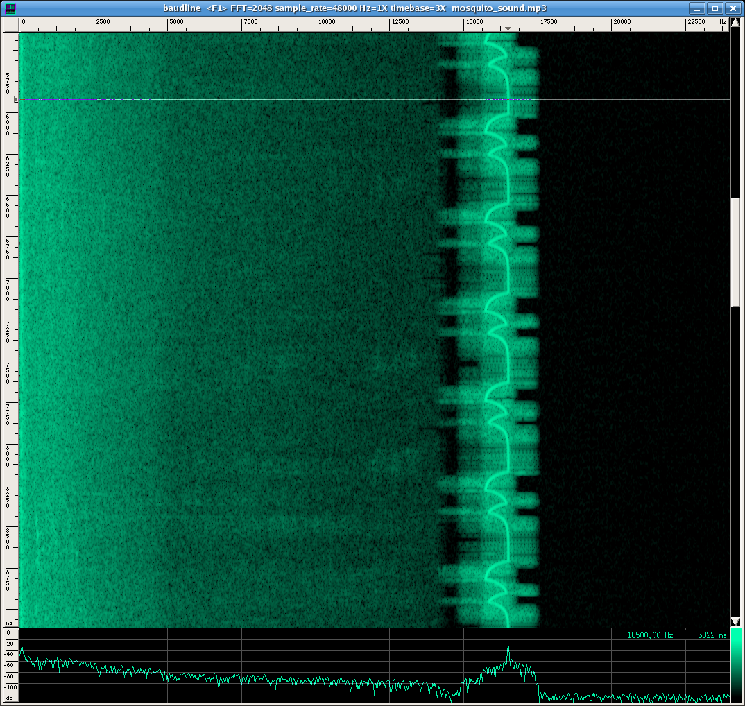
The baudline ultrasonic analyzer was used to examine the MP3 Mosquito sound file at the end of the article. The spectrogram is below:



Background road noise is visible on the left side of the spectrogram. The right side shows a strong tone that sweeps between 15700 and 16500 Hz. The attack and decay slopes have a typical RC shape. The fact that the Mosquito tone is sweeping probably makes it more effective than a stationary tone would be. The human brain is very good at notching out and ignoring constant tones like NTSC or PAL retrace emissions. A moving tone that looks a lot like a siren demands attention.



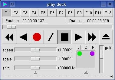
Baudline's Play Deck can be used to transform the Mosquito sound into an audible signal for those whose hearing is attenuated above 15kHz. Try slowing the playback down .5X to .25X speed. Or try shifting the signal down about -10000 Hz. The shift slider is equivalent to down mixing which makes it like a radio tuner for audio signals.

An ironic twist has developed, the Mosquito ultrasonic tone is now being used by teenagers as a cell phone ring tone. Most schools require that cell phones be turned off in class rooms and since most teachers can't hear that high in frequency the ringing can go undetected.

What is next in the ever changing Mosquito ultrasonic technological battlefield? Baudline spectrum analyzers in the classroom? It is a possibility. Contact us if you are interested!

Big Bang Acoustics

The Big Bang is a scientific theory that describes how the universe began from nothingness some 13.7 billion years ago. It started with a silent explosion of matter and energy. This incredible cosmic event was completely silent since there wasn't anything to radiate sound into. After the universe expanded and cooled slightly the physics of pressure were allowed to act. Where there is pressure there can be sound, and the universe began to sing.

Two physicists have created slightly different Big Bang acoustic models of the first million years. Both mathematical simulations utilize the cosmic microwave background (CMB) radiation data from the WMAP survey project. This CMB data is a glimpse back into time at the early universe's density variations. The changes in density became clumps and nulls which attracted and reflected pressure variations in the hot primordial gas. This was sound and it had a spectrum. Both mathematical simulations use this base spectrum as a starting point to extrapolate into the future and the past. They attempt to answer the question of what the Big Bang and the expanding universe might of sounded like.

The baudline scientific visualizer was used to analyze these two Big Bang acoustic models.

Cramer
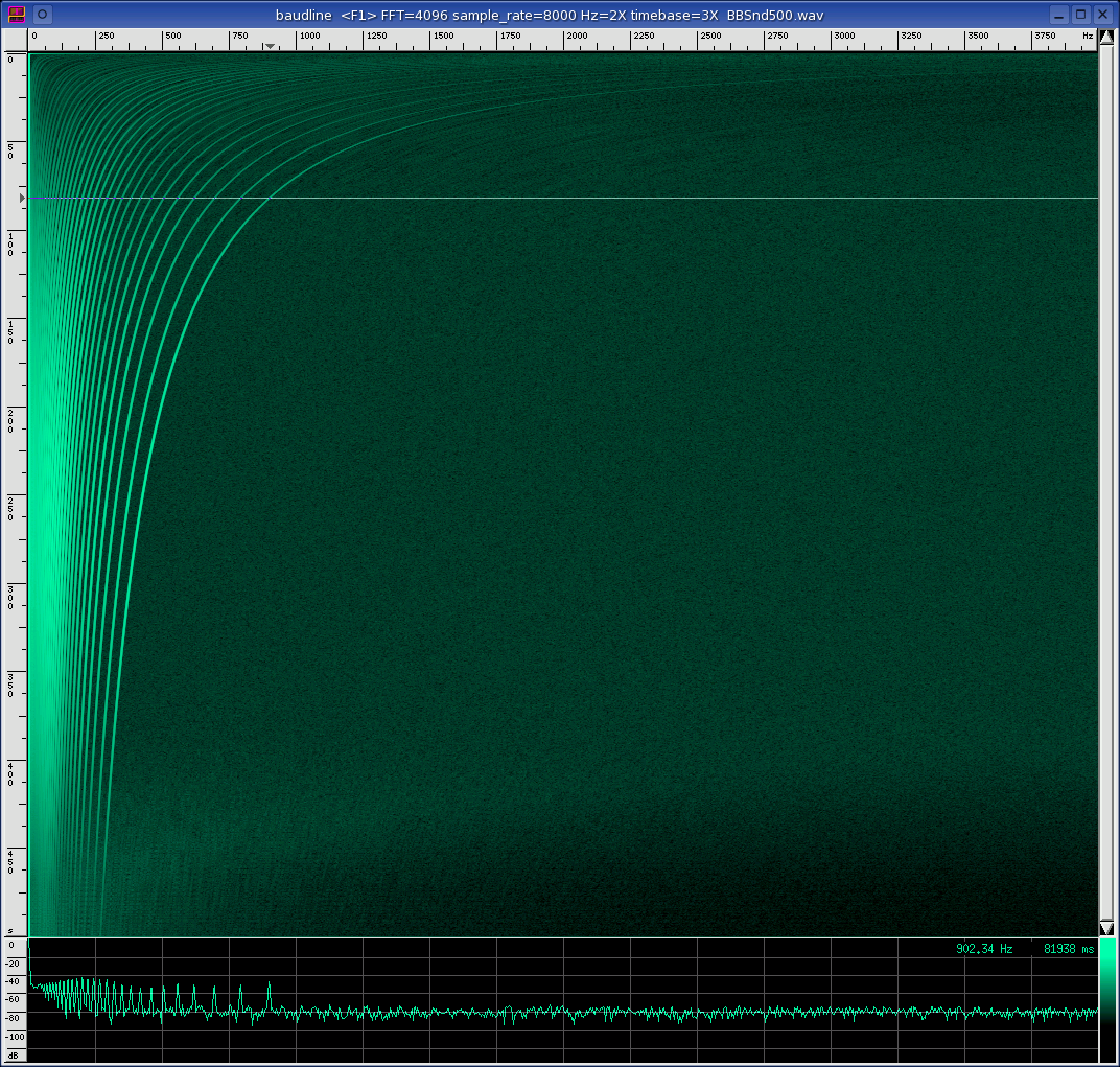
John G. Cramer, Professor of Physics at the University of Washington, used a Mathematica program that generated the sound of the universe's first 760,000 years. He used the WMAP microwave data as input and the formula time^2/3 that approximated the rate of growth of the expanding universe. The frequencies of Cramer's simulations have been increased by a factor of 10²⁶ so that they would be in the audible range.

The .wav data files, description of the simulation technique, and an explanation of the physics involved can be found here:

• BOOMERanG and the Sound of the Big Bang paper
  
• recap, linkbacks, and larger data files
  

The spectrogram of Cramer's model of the universe's first 760,000 years is below:



The above spectrogram shows a universe that is rich in harmonic content. It begins as a downward exponential sweep that decays into a hiss like noise at the end. Cramer says in the afterword of his paper that "the spectrum of frequencies at which the universe was acting as a resonator has been well measured by BOOMERanG and more recently by WMAP." The strong spectral peaks correspond to a resonating structure.


Whittle
Mark Whittle, Professor at the University of Virginia, used the WMAP data to model the sound of the universe's first million years. The sound has been transposed up by 50 octaves so that it is in the audible range. A 50 octave increase is equal to the frequency being multiplied by a factor of 2⁵⁰. The sound of the Big Bang was extremely low bass.

The .wav data files, description of the simulation technique, and an explanation of the physics involved can be found here:

• Primal Scream presentation
  
• data files, descriptions, diagrams
  

The spectrogram of Whittle's model of the universe's first 1,000,000 years is below:



The above spectrogram shows a white noise like universe with harmonic rich nulls that exponentially sweep downward in frequency. At the 500,000 year point the higher frequencies transform into high frequency noise. The Whittle model looks a lot like the Cramer model except instead of pure clean tones there are deep nulls.



What is interesting about the spectral nulls is that they look a lot like room mode acoustics where the wall dimensions determine which frequencies are boosted and which are attenuated. To carry this room mode analogy a little further would suggest that the exponential downward sweep is the result of the walls being pushed apart until the 500,000 year point where the walls dissolve allowing any built up frequencies to slowly diffuse. The tangential modes of a cube shaped room would match this spectrum almost exactly but the axial and oblique modes, although weaker, would add extra non-harmonic spectral content. Fortunately a sphere symmetry can be modeled as a cube with only tangential modes.

Harmonics
The harmonic structure from the Cramer and Whittle models are very different. In fact they do not have integer ratios and they are not true harmonics at all.

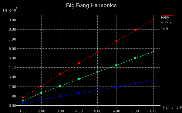
The fundamental of the Whittle modes is an oddball null being strangely offset (see spectrum above). All of the other Whittle harmonic nulls line up nicely if a phantom fundamental is used. Try using baudline's harmonic bars tool to get an interactive feel for this. Below is a frequency vs. harmonic number plot of the Whittle data that shows a straight line relationship, so the first null is on the line but it is not part of the harmonic progression. Not sure if this anomaly is part of the WMAP data or if it is a simulation artifact. If it is a real and accurate phenomena then it opens up a number of intriguing possibilities and questions.




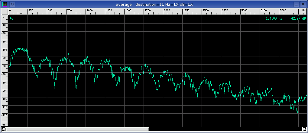
The Cramer spectrum at first looks harmonic in structure but closer examination shows an increasing frequency progression that is almost log like. See the average spectrum below:



Conclusion
The Cramer and Whittle models are as similar as they are different. They are both interpretations of the same WMAP data and they both demonstrate an almost 14 billion year old sound of the expanding universe. Saying which model is correct is a difficult, if not impossible, task. I can't wait to hear what new data and future physics discoveries might reveal.

VLF whistler echo train

The baudline VLF analyzer was used to investigate a whistler natural radio emission signal file from the NASA INSPIRE VLF project web page:

http://image.gsfc.nasa.gov/poetry/inspire/advanced.html

A whistler is an atmospheric electrical event that has traveled a very long distance. Usually a whistler is sent out into space and is curved back to earth along magnetic field lines. This long distance allows for a large amount of frequency dispersion which causes a lot of curvature. The original sferics wideband pulse is bent into what looks like an exponential downward sweep.

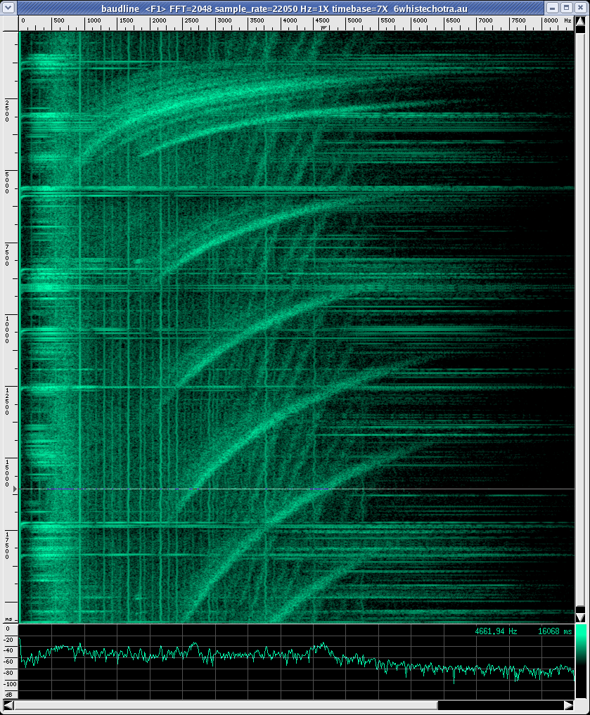
On the advanced INSPIRE VLF page is a whistler echo train signal file called 6whistechortra.au. It is consists of a primary whistler event and six echoes that are clearly visible in the baudline spectrogram image below:




The NASA INSPIRE page says:

"Echo trains result when the radio wave bounces back and forth between magnetic conjugate points. Each time the signal bounces off the ionosphere, some of the energy leaks down in the lower atmosphere and is heard as a whistler. All of the whistlers in the train are the result of a single lightning stroke. Successive "hops" of the whistler are seen with increasing dispersion time as the distance traveled grows with each bounce."

This increase in dispersion time can be seen in the spectrogram as the whistler echoes becoming increasingly bent. The lower frequencies travel slower than the higher frequencies. What's interesting is how uniform the dispersion is as a function of frequency. Baudline's periodicity measurement bars are a perfect tool for investigating this phenomena. A frequency point on the exponential whistler curve is chosen and then the periodicity bars are stretched and dragged to make the measurement. See the baudline spectrogram image below: (click image for a clearer view of the periodicity bars)




This delta delay varies from 3.1 seconds at about 5300 Hz to 4.5 seconds at 2200 Hz. The periodicity bar measurements line up perfectly at every frequency so these are true echoes and the delta delay is a function of frequency.

The speed of light is about 300,000 km/sec (186,000 miles/second). The shortest whistler echo delay at the highest frequency is 3.1 seconds. So if a constant speed of light whistler velocity is assumed, which it isn't, then the distance traveled equals 930,000 km. The Earth - Moon distance is 384,000 km, so the whistler echo distance traveled is roughly equal to a circular path (diameter * pi) to and from the Moon. This is just speculation and without more detailed information about the whistler echo recording it impossible to say for certain that an Earth - Moon circular path is happening. What is known is that the whistler echoes are traveling a very long distance.

Another interesting observation is by the time of the 4th echo return that the high frequency head of the signal has caught up with the low frequency tail and passed it. The whistler thickness is also increasing with each subsequent echo, so given enough duration, the exponential whistler will dissolve into white noise (equal energy at every frequency) and become spectrally flat.

Fascinating. A lot of physics is going on in this whistler echo train signal.