
This Voyager signal was recorded at 8419.62 MHz and was packetized into an .archive-compamp file by SonATA. The following command line streams the 4-bit quadrature Voyager samples into baudline:
cat 2012-11-07_21-14-05_UTC.act61.dx1011.id-4.L.archive-compamp | extract_compamp_data 9 | baudline -session compamp -stdin -format s4 -channels 2 -quadrature -samplerate 711.1111 -record
This Unix command line of multiple pipes extracts the 9th channel from the .archive-compamp file and feeds that into baudline's standard input with the appropriate configuration settings. Note the .L. in the compamp file name. I don't know why SonATA does this but the X & Y linear polarization .compamp files are labeled as being L & R circular polarization.
X polarization
Below is the baudline spectrogram of the X linear polarization. Note the weak diagonal signal on the left side that starts on the top at around -160 Hz. This drifting line is caused by the Earth's rotation and the Doppler Effect. I call it Doppler Drift. Click on the image below for a larger and better view of this weak signal.

Y polarization
Below is the baudline spectrogram of the Y linear polarization file. Note that the signal is bit stronger than it was in the X polarization above. Compare this with the signal strength from the July 2010 Voyager data analysis.

X & Y polarizations
The two spectrograms above were combined to create this dual channel spectrogram (see the Channel Mapping window). The X polarization is green and the Y polarization is purple. Notice how this dual channel technique makes the weak drifting Voyager signal easier to see. It also makes it easy to visually compare both polarizations.

If you click to look closely at the larger version of this image you'll see several very weak crisscrossing lines and curved whistler-like shapes that are much weaker than the main drifting signal. These very weak features could be real or they could be just random shapes in the noise floor. Need more data to know for sure. If they are real then they're likely artifacts caused by distortion somewhere in the signal path.
Auto Drift
Baudline's Auto Drift feature was enabled and each of the X & Y polarizations were pasted into the Average window. The Y polarization (purple) is about half a dB stronger which confirms our spectrogram strength observation mentioned above. The drifting signals are about 3 - 4 sigma above the noise floor. The auto drift rate measurement window reports that the signal is drifting by -0.5770 Hz/second.

Next Auto Drift is enabled with baudline's spectrogram display. Think of this as a 4-dimensional version of the above Average display where the additional dimensions are time and vector space. Each pixel has 20865 possible vector paths and that works out to about 10 billion possible vector paths seen in the spectrogram image below. Good thing that Auto Drift is a quick O(n log n) algorithm so that image rendering is rather fast. For reference the Drift Integrator's settings were: beam width = 326 slices (16 seconds), optimum overlap = 400%, Auto Drift quality = 8.

Notice how the weak drifting signal stands out and is easier to see. Also note how the drifting signal fades in strength between the X (green) & Y (purple) polarizations. This image reminds me a lot of ice crystals on a window pane. It isn't that far out there since the Auto Drift algorithm that generates the spectrogram vectors is somewhat similar to how ice crystals grow.
Histogram
The Histogram window shows 5 vertical lines (bins) that make a Gaussian-like shape (see AWGN). This sparse histogram is not surprising since the input signal has 4-bit quantization. Note that only slightly more than two bits are being utilized.

Waveform
Baudline's Waveform window shows a time series view of what the 4-bit quadrature signal looks like. This sample distribution matches what is seen in the Histogram window above. Do you see the signal? It's the magic of DSP that allows such a weak drifting signal to be encoded in so few bits.

Conclusion
No modulation characteristics are visible in either the baudline spectrogram or Average window views. The Voyager signal looks like a non-information baring pilot tone. This could be due to the weak nature of the signal or because Voyager was not transmitting at the time the signal was recorded.
As mentioned above, this setiQuest Voyager 1 redux capture is much weaker than the July 2010 Voyager 1 signal I previously blogged about. A good question is why is it weaker? Here is a list of possible explanations:
- 28 months have passed and Voyager is now 8.3 AU farther away.
- Voyager has entered the Heliosheath and the compressed turbulent solar wind is increasing signal attenuation.
- Voyager's Plutonium-238 power plant has a half-life of 88 years and is producing less power for signal transmission.
- Voyager's dish antenna could be slightly off axis and is not pointed directly at Earth.
- The ATA dishes could be slightly off axis and are not pointed directly at Voyager.
- Reduced collection area due to some ATA dishes being off-line.
- Some cryo feed units require maintenance and are resulting in a higher ATA system temperature.
- An error in the calculation of the ATA beamformer coefficients.
- Increased local RFI mixed with Walshing artifacts are effectively reducing ATA system gain.
- Rainy cloudy weather in Hat Creek, California.
- The compamp 4-bit sample quantization is pushing up the noise floor. The first Voyager data collection used 16-bit samples.
- Aliens have found the Voyager space probe and are fiddling with its innards.
Links
- http://setiquest.org/forum/topic/baudline-analysis-voyager-1-redux
- http://baudline.blogspot.com/2011/03/setiquest-voyager.html
- http://voyager.jpl.nasa.gov/
- http://www.nasa.gov/vision/universe/solarsystem/voyager_agu.html
- http://twitter.com/NASAVoyager
- http://twitter.com/NASAVoyager2
Software licensed through SigBlips.